Sometimes, Excel seems too good to be true. All I have to do is enter a formula, and pretty much anything I'd ever need to do manually can be done automatically. Need to merge two sheets with similar data? Excel can do it. Need to do simple math? Excel can do it. Need to combine information in multiple cells? Excel can do it. In the spirit of working more efficiently and avoiding tedious, manual work, here are a few Excel tricks to get you started with how to use Excel.
Add Secondary Axis
Method 1
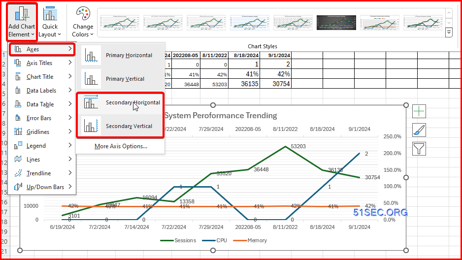
Method 2
You can choose Plot Series on
- Primary Axis
- Secondary Axis
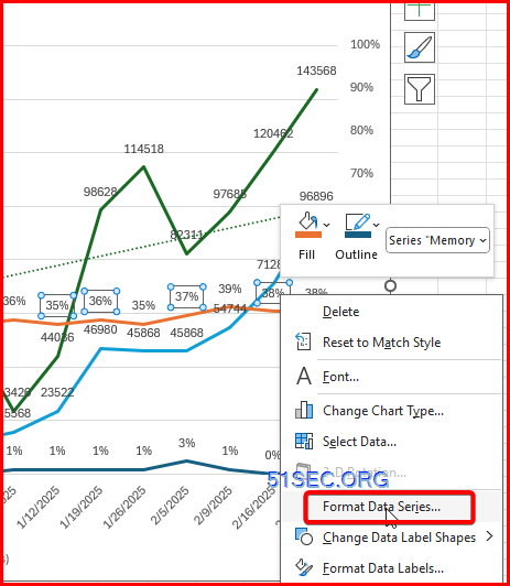
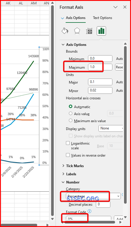
Format Secondary Axis
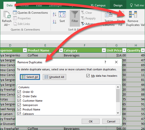
Remove Duplicates
Keyboard shortcut: Alt+A+M
This brings up the Remove Duplicates window where we can select which column(s) we want Excel to remove duplicates from.
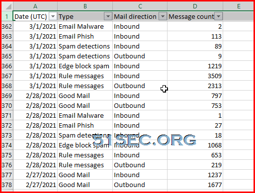
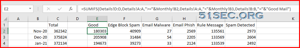
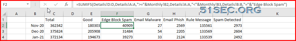
Sum for certain month based on conditions
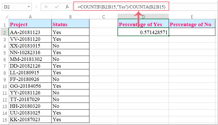
Count Word Appear Percentage
Enter this formula: =COUNTIF(B2:B15,"Yes")/COUNTA(B2:B15) into a blank cell where you want to get the result, and then press Enter to a decimal number, see screenshot:
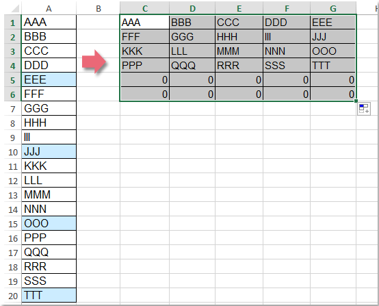
Transpose Every 5 Or N Rows to Columns
Transpose Every 5 Or N Rows From One Column To Multiple Columns With Formula
In Excel, you can apply the following formula to transpose every n rows from one column to multiple columns, please do as follows:
1. Enter the following formula into a blank cell where you want to put the result, C1, for example, =INDEX($A:$A,ROW(A1)*5-5+COLUMN(A1)), see screenshot:

Note: In the above formula, A:A is the column reference that you want to transpose, and A1 is the first cell of the used column, the number 5 indicates the number of columns that your data will locate, you can change them to your need. And the first cell of the list must be located at the first row in the worksheet.
2. Then drag the fill handle right to five cells, and go on dragging the fill handle down to the range of cells until displays 0 , see screenshot:
Copy Web Page Data into Excel
For example, copying following page into excel is a mess.

Here is what I did:


Open Excel files in New Window
- In Excel 2003, go to Tools -> Options -> General tab. Make sure the option, ‘Ignore other applications’ is checked.
- In Excel 2007 & 2010, Click the Office button -> Excel Options -> Advanced. Under General, check ‘Ignore other applications that use Dynamic Data Exchange’.
Formula- Convert a text to Number
Search a Column of Strings Based on Data in another Column
=MATCH("*"&(O6)&"*",B:B,0)
Matching and Return value crossing different columns
=IF( COUNTIF('Servers'!A:A, A3)=0, "No", "Yes")
Check if A3 value is in worksheet "Servers" column A. If found , show Yes, else, show No
Check if A3 value found in the file "Z:\0 Operation\1 Scan\[Scan_Report_Server.xlsx" - worksheet "APP IP' - Column A to H. If found, return same row's , eighth column's value.
Pivot Table Tips
1 Put Multiple Columns into Pivot Table
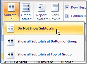
2 Do not show subtotal from Pivot Table
After you enabled Classic Pivot Table layout, by default, subtotal will show . Here is how to turn it off:
Step 1. Select a cell in the pivot table
Step 2. On the Ribbon, click the Design tab
Step 3. In the Layout group, click Subtotals, and click Do Not Show Subtotals.
3 Change PivotTable Column Name
Excel GIFs
Automatically Add Column Titles on Each Print Page:
Set Tables Border:
用数据透视表做分组计数
填色Out了,Excel这样的“自动提醒”更实用!
excel自动提醒功能,在实际工作中很常用。大多是通过填充颜色的方式设置提醒。今天学习的则是一种更直观的方法:用漂亮的图标。
【例】如下图所示A为到期日期(今天日期是2018-1-7),要求在B列设置到期提醒,规则如下图右表所示。
B2公式:=a2-today()

操作步骤:
1.选取B列区域,开始 - 条件格式 - 新建规则

2.在打开的新建规则窗口中进行如下图所示设置
- 规则类型:默认
- 格式样式:图标集
- 图标样式:黑红黄绿4按钮格式
- 设置区间值:根据需要填写间隔值
- 类型:默认是百分比,这里改成数字。

设置完成!效果如下:

注:很多益友一定很好奇E列的图标是怎么输入进去的,其实道理一样的,只需要在E列随意输入C列区间的任意数字,然后设置图标显示,再只显示图标就OK了。

有了这样一个到期提醒表,以后再也不用担心因到期未处理会带来损夫。条件格式功能真的帅呆了!
会动的图表 Excel让数据开始说话!
Excel图表数据最给人最大的感觉就是,密密麻麻,虽然有柱状图表示内容,看起来似乎清晰明了,但是看起来不够直观,尤其数据较多的时候,如何能够在有限的屏幕宽度内浏览更多的数据呢?不放让数据动起来吧!

打开Excel,在要制作成动态数据表格的页面上切换选项卡到开发工具(如没有开发工具,请点击Excel文件—选项—自定义功能区,右侧勾选开发工具即可),选择“插入”表单控件中的滚动条。


右键单击滚动条,选择设置控件格式。

切换选项卡到“控制”一项,修改单元格链接,比如我们选中的是E9这个空白单元格(点击单元格链接后的小图标可以直接选择单元格)。

这时,按下Ctrl+F3打开名称管理器,这里略复杂,弹出的窗口是新建自定义名称,第一个比如叫日期,就输入
=OFFSET(Sheet1!$A$1,Sheet1!$E$9,,5),第二个比如叫数据,一样输入=OFFSET(Sheet1!$B$1,Sheet1!$E$9,,5),实际上就是这两个名称的位置定位。这里的意思是,OFFSET函数的行偏移量由E9单元格指定,而E6单元格则由滚动条控件来控制,这样每单击一次滚动条,OFFSET函数的行偏移量就会发生变化。


现在开始制作图表,在Excel界面选择“插入”选项卡,找到折线图的小图标(在推荐的图表附近),点击选择一个折线图。

在刚刚建立的图表数据上右键单击,选择“选择数据”。

在选择数据源中分别编辑左侧图列项(系列)和水平(分类)轴标签,分别对应之前修改自定义名称(日期、数据)。


最后,再根据实际需求,修改图表高度、单元格高度,并辅以底色之类的美化工作,最终,就能依靠滚动条让图标数据动起来,实现动态数据浏览了。


![[5 Mins Docker] Deploy FreshRSS Using Docker Run Command and Deploy To Fly.io](https://lh3.googleusercontent.com/blogger_img_proxy/AEn0k_tAdBMT3ZuCOwnQVLPOduyONJfLOu39ZYerlxZDk4lNB8mWfVjs67zubenVZWiEhJszFd0lNiKmkplgXkSWtZBe0mHJ_A9Pwih_MowRwF6ntg)


No comments:
Post a Comment